Expectations, Tails, and Poisson-Gamma

Every game starts with an initial set of rules and assumptions. In the world of sustainable and iterative multiplayer games, these rules are crucial. They outline a framework and create incentives that allow players to co-exist and progress as they engage with one another and the game. For the purpose of this article, I’ll focus on those initial assumptions that are unique to each player. These assumptions give each player the freedom to interpret the rules in their own way, staying within acceptable limits. This raises a natural question: how often should a player update their assumptions about potential future levels they might want to explore? Conversely, is it even necessary for the player to update their assumptions at all?
In my article titled “Gradient Ascent, Global Maximum, and Complexity,” I shared some observations based on simulations I conducted. One key takeaway was that just because a player’s strategy works well for one level, it doesn’t necessarily mean it will work for higher and more complex levels. As such, you may rightfully state that just based on this statement, I fall under the camp of updating expectations as the player progresses through the game.
Let’s explore how this idea fits within a framework of jump events. In my article titled “Continuity, Jumps, and Measuring Progress,” we discussed how progress in life can be approximated by a jump diffusion process. Specifically, I outlined that while incremental progress happens almost continuously, there are significant “jumps” that make your progress quite evident.
For this thought experiment, I’ll suggest that decay in performance might also follow a similar jump diffusion process. This means that while a player’s performance may gradually decline over time, there can be sudden, noticeable drops that highlight this decline. Given the well-known concept of loss aversion in behavioural economics, I think that it becomes even more crucial to understand if updating expectations in the face of significant loss events makes sense.
In trying to look for a good example to illustrate this, I stumbled upon the Poisson-Gamma model that provides a framework for updating expectations for defaults on observed data. Before we dive into the model, I do want to touch upon the Poisson Distribution and Gamma Distribution momentarily.
Poisson distribution: The Poisson distribution is a discrete probability distribution that models the number of events occurring within a fixed interval of time or space, assuming that these events happen independently and at a constant rate. It is characterised by a single parameter λ, which represents the average rate of occurrence of events.
Gamma distribution: The Gamma distribution is a continuous probability distribution that models positive real numbers and is often used to model waiting times or the time until an event occurs. It is characterized by two parameters: the shape parameter α and the rate parameter β.
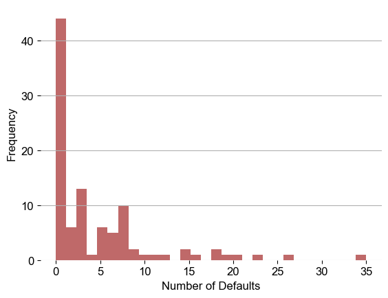
We can now begin with our experiment. Across multiple discussions, we’ve established that we are operating in a world with outcomes from a distribution with heavy tails. As such, let’s simulate some synthetic default data that showcases extreme outcomes. We can start by setting up the initial parameters for our Gamma (prior) distribution. These parameters reflect our prior beliefs about the rate of defaults before observing any data.
# Parameters for extreme outcomes
alpha = 0.5  # Smaller alpha for more variability
beta = 0.1   # Smaller beta for more variability
n_periods = 100

# Generate Gamma-distributed rates with extreme values
lambda_vals_extreme = np.random.gamma(alpha, 1/beta, n_periods)

# Generate Poisson-distributed defaults with extreme rates
defaults_extreme = np.random.poisson(lambda_vals_extreme)
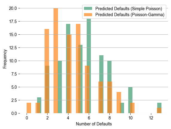
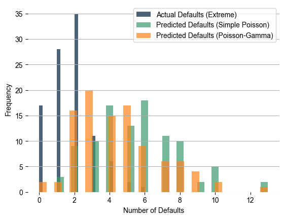
Next, we dive into simulations for the default rate. By using the simulated λ values above, we then simulate the number of defaults from the Poisson distribution. Further, with this simulated data in hand, we update our Gamma Distribution parameters, which allows us to simulate the posterior distribution for λ. Using these values, we simulate future defaults, capturing those extreme outcomes. For comparison, we also simulate defaults using a simpler Poisson model, where the rate is fixed at the mean of observed defaults.


The Poisson-Gamma model, comparatively, captures a broader range of possible outcomes, including more extreme defaults. Its strength lies in its flexibility to adjust parameters based on observed data.
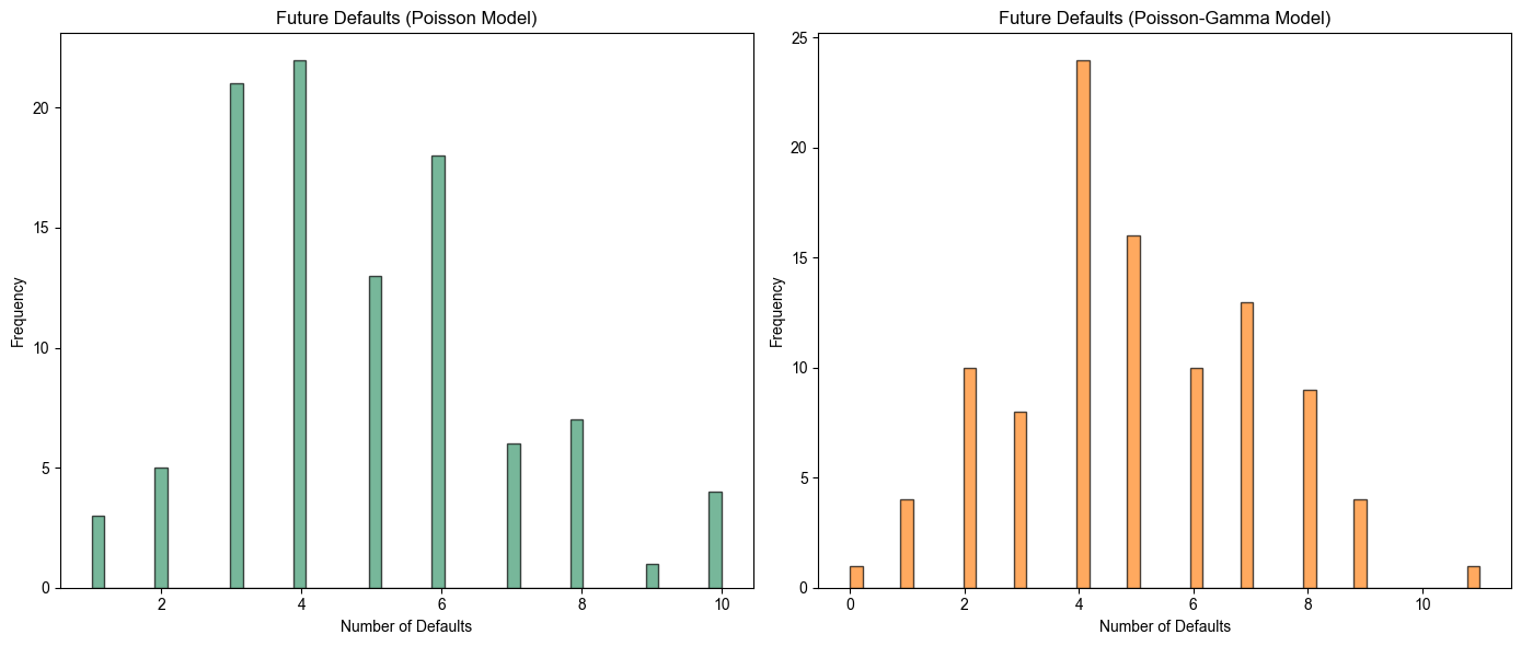
Now, let’s flip the script. What happens if the variability in the underlying population isn’t too high or the if the training dataset is too small? Below, you’ll see the mean and variance of predicted outcomes between the two models. Here, the simpler Poisson model outperforms the Poisson-Gamma model in exhibiting less variance while still closely matching the mean rate prediction.

Actual default rate: 5.0
Poisson Model - Mean: 4.84; Variance: 4.17
Poisson-Gamma Model - Mean: 4.94; Variance: 4.78
Based on these simple experiments, we’ve learned something that might seem obvious at first glance:
-
In situations where the underlying jump event shows high variability in both frequency and severity (think of our player navigating a world full of unknown unknowns), it makes intuitive sense to model our expectations using parameters that we update regularly.
-
On the other hand, when the underlying event is stable and predictable, introducing the complexity of a Gamma component may be unnecessary. It brings to mind the old phrase “if it ain’t broke, don’t fix it”—essentially, if something has been working well for a long time, there’s likely a good reason for that success, even if we don’t fully grasp it at the moment.
As for how often we should update our assumptions if we find ourselves in environments that we know are full of unknown unknowns, that’s a tougher question. In a previous article here, I highlighted that when a player starts using significantly more resources (like increased computational time) to achieve the same progress, it might indicate they’ve “leveled up.” Perhaps this could also signal the right time to update our assumptions and parameters in preparation for upcoming challenges in the game?
One key takeaway from this thought experiment is that as an active participant, the player first needs to determine whether they are operating in a highly variable environment. This initial assessment is crucial because it guides how often (or even if) parameters should be updated—a decision that comes only after understanding the game’s variability.
Before getting into the nitty-gritty of updating parameters, it’s important for the player to have a clear grasp of the current state of the game and to envision its potential future.